Data Transposition in MS Excel

After entering data into your spreadsheet, you may find that the data would be better organized in a different format. You could wish to convert columns to rows or vice versa. This tutorial demonstrates two approaches for transposing data in Microsoft Excel.
To transpose data, use Copy and Paste Special.
Using the Paste Special tool in Excel is a simple approach to transpose data. You can, for example, copy data from a column and paste it as a row without manually relocating the column data.
- Choose the data to be transposed. Just move your pointer between the cells to accomplish this.
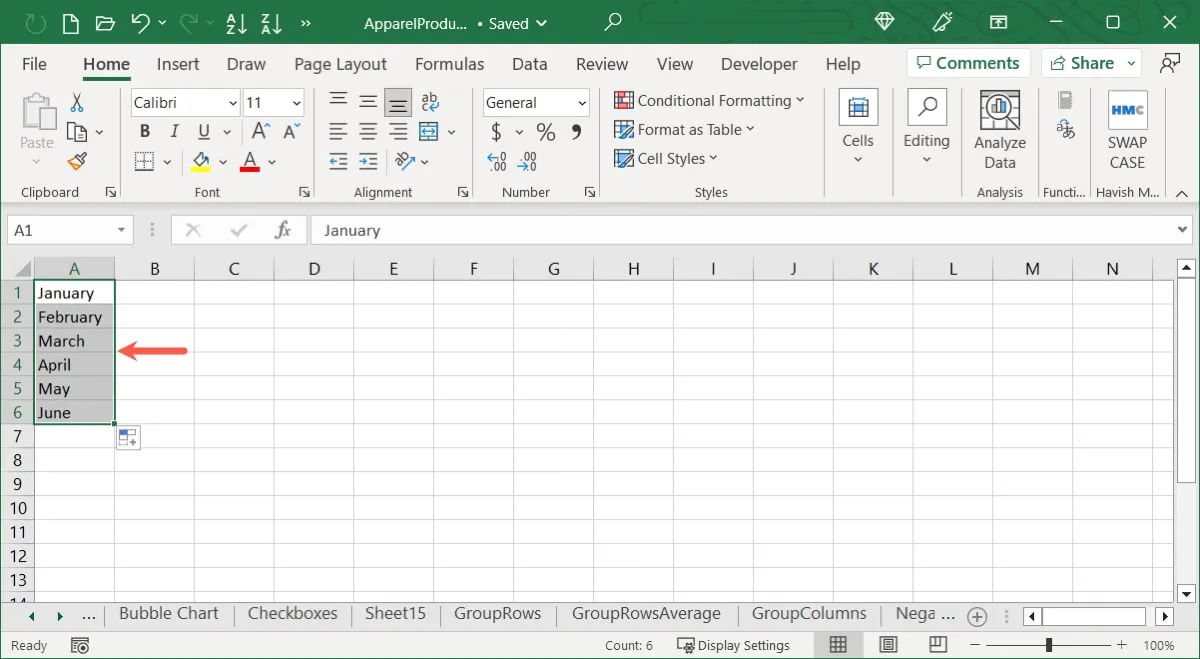
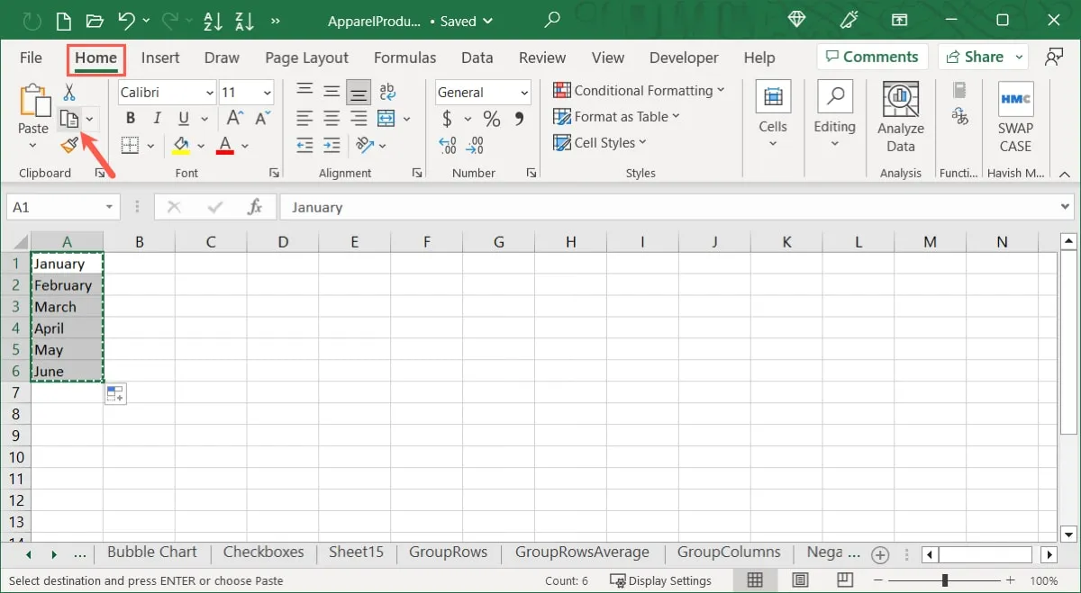
- Right-click one of the chosen cells and select “Copy,” or click “Copy” in the Clipboard area of the “Home” tab’s ribbon.
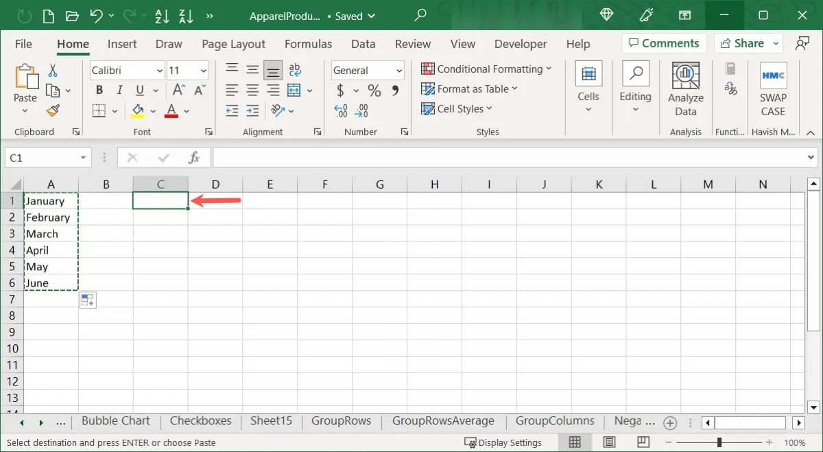
- Choose the first cell where you want the data to go. You should select a separate location on your sheet that is not on top of the existing data. This eliminates mistakes and allows you to validate that the data is appropriately transposed without overwriting any data.
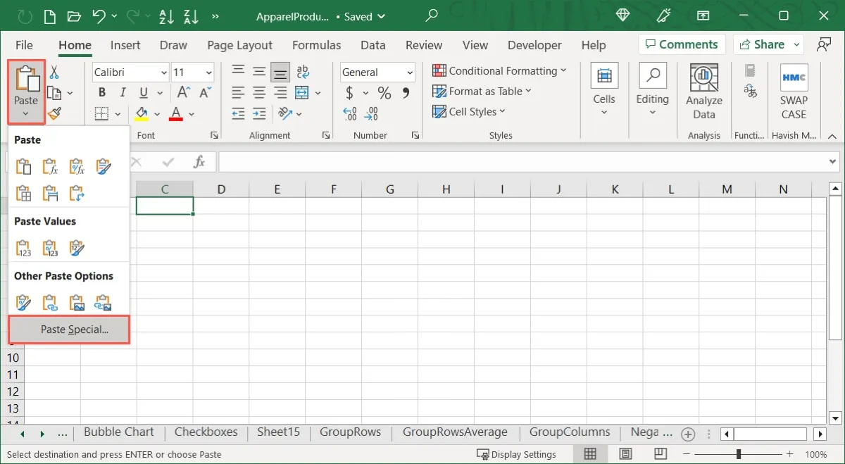
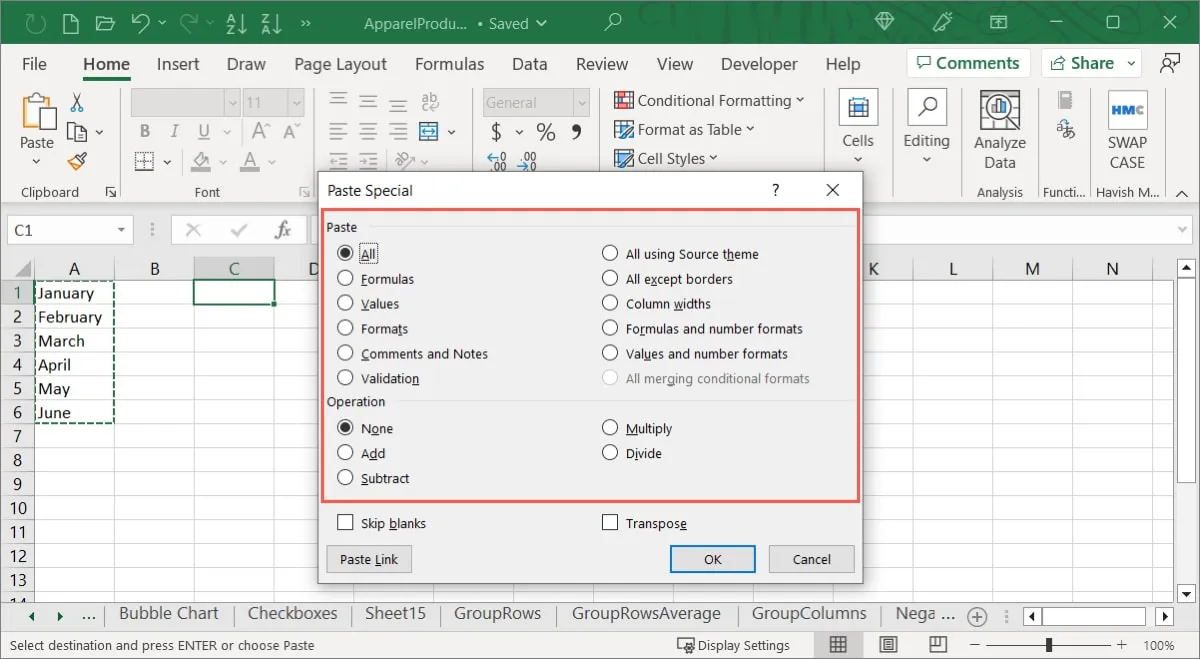
- Right-click the cell, choose “Paste Special,” and then pick “Paste Special” from the pop-up menu, or click the “Paste Special” drop-down menu on the “Home” tab and then select “Paste Special.”
- If you like, you may pick a specific “Paste” option at the top of the Paste Special box. Choose “All” to paste the data exactly as it is. If you wish to add or delete data from the pasted data, you may pick a “Operation” towards the bottom of the box.
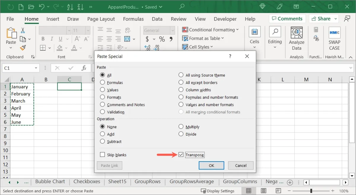
- Check the “Transpose” box at the bottom of the box and click “OK” to paste the data.
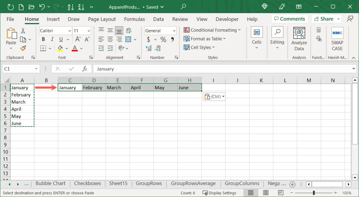
- Depending on your choices, your data will be pasted from a column to a row or vice versa. If you choose, you may then delete the original data.
In Excel, use the TRANSPOSE Function.
The TRANSPOSE function in Excel may also be used to transpose data. This option operates similarly to the previous operations; however, you may utilize the function to transpose table data if necessary. This is a current restriction of the Paste Special Transpose capability.
The formula syntax is TRANSPOSE (range), where the cell references for the range or array to be transposed are entered.
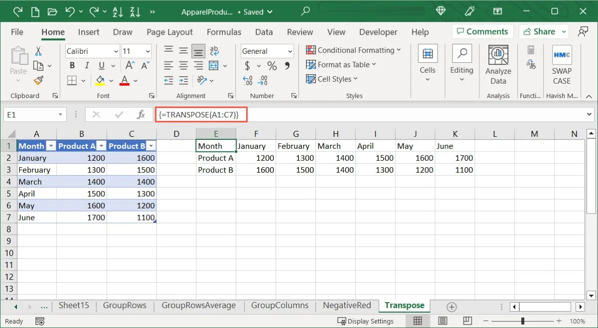
- Enter the TRANSPOSE function formula after selecting the initial cell where you wish to insert the data. Transposing the range A1 through C7 from our database as an example. Here’s how it works:
=TRANSPOSE(A1:C7)
- When you see the preview in Excel for Microsoft 365, hit Enter.
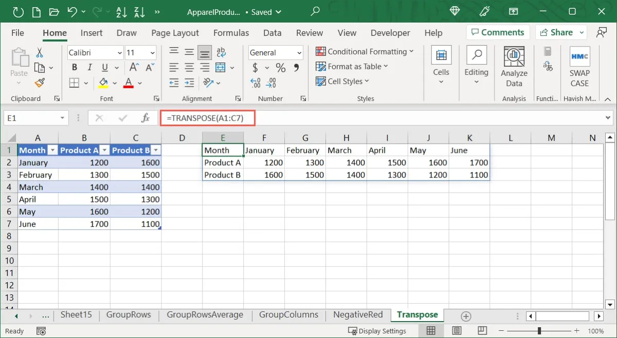
- If you’re using a different version of Excel, use Ctrl + Shift + Enter to wrap the formula in curly brackets since the function utilizes an array formula that isn’t supported in the same manner across Excel versions.
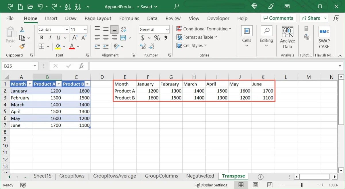
- The column data will be put in a row or vice versa. You can delete the original data using the same technique as described earlier.
Frequently Asked Questions
Do formulas automatically update when I transpose data?
When you utilize relative references for your data, the Excel formulae update automatically utilizing the two transposition approaches described above. If you utilize absolute references, however, the formula may not update as expected or may create problems.
Can I transpose filtered data in Excel?
If you have filtered data that you wish to transpose, use the Paste Special option. Although you may use the TRANSPOSE function for the formula by choosing only the visible, filtered cells, the output will most likely be inaccurate.
How to I undo transposing data in Excel?
If you transpose the data using one of these approaches and then determine that the original manner worked better, you may undo the modification. To undo many activities, use the “Undo” button in the Quick Access Toolbar or open the “Undo” button’s drop-down menu.
Keep in mind that after you save and close the Excel file, the Undo option for previous operations is no longer available. In this situation, you may use the original procedure to transpose the data in reverse.
Image credit: Pixabay. All screenshots by Sandy Writtenhouse.


Leave a Reply