Excel’s ISNUMBER function explained and how to use it

The ISNUMBER function in Microsoft Excel is an information function that tests if a certain cell has a specified value or not. It does this by determining whether or not the cell contains the value. This operates correctly on texts as well as numbers and returns either the result YES or FALSE depending on the outcome.

Although though this is a relatively simple function, it may be used in conjunction with a number of other functions, such as Search, if, and so on, to construct sophisticated algorithms and then apply those algorithms in Excel. The ISNUMBER function, when used by itself, gives you the ability to check the value that is contained within a cell or a group of cells.

Excel’s ISNUMBER function explained and how to utilize it

Excel’s ISNUMBER function enables users to conduct conditional formatting on cells that contain numbers and detect whether or not the desired value has been reached. Let’s say, for instance, that you only want a Cell to be filled in when the value being entered is a number.

If the item being checked is a number, then the ISNUMBER function will return the value TRUE, but if it is not a number, then it will return the value FALSE. You may use this function to check whether or not a value is a number. Follow these steps in order to make use of this function in Microsoft Excel:

• To begin, launch Excel and launch either a brand new or an existing spreadsheet.
• Now go ahead and choose the cell in which you would like the outcome of this function to appear.
• In this cell, type the following, and then change the value that is enclosed in brackets with the reference to the cell where the value you wish to test is located or the value itself.

=ISNUMBER(value)

• If, for instance, you wish to determine whether or not a certain Cell has any integers, you may use the following piece of code:

=ISNUMBER(C5)

• When you press Enter, if there is a number stored within that Cell, you will see the word “TRUE” display on the screen.

• In the event that there is more content within the specified cell, this operation will return the value false.

While performing conditional formatting, users may also utilize this ISNUMBER function in conjunction with the IF function to get the desired results. This function can also be used with other functions, such as those from other packages, to produce more complicated equations.

Excel tutorial on how to locate the ISNUMBER function.

You may make use of any one of the following three methods to put this function in Excel to work for you. Nevertheless, before you do anything more, you need to be sure that you have selected the particular Cell in which you want the result to appear. Assuming that you have previously chosen a Cell to work with, proceed with the steps below:

• On the actual Cell, you should begin entering “=ISNUMBER()” without the quotation marks.
• Click the Formulas tab, then pick Additional functions from the drop-down menu. Click the Information > ISNUMBER option that appears when the drop-down menu does.

• The fx key can also be used to access this ISNUMBER function as an alternative option. Check out the Snapshot that we have below

Once the function arguments window has opened, you should start typing the ISNUMBER function with the “=” icon, followed by the parameter that you want to check up. When you have clicked the OK button, the result will be shown in the Cell that has been chosen.

With conditional formatting, how do I utilize the ISNUMBER variable?

As was just said, the ISNUMBER function in Excel may be utilized in order to carry out various forms of conditional formatting. Well, here’s how it works:

• To begin, fire up Microsoft Excel and enter all of the required data into the appropriate cells.
• Make sure that all of the cells that you want to apply the conditional formatting to are selected.
• Now, choose the Home tab, and then under the Styles subheading, select the Conditional Formatting option.
• When a menu with drop-down options appears, pick “New Rule.”
• You will now be sent to a new window that will walk you through the process of implementing six distinct rules.
• Choose the Rule type “Use a formula to select which cells to format,” and then click the “OK” button.
• In the field labeled “Format values where this formula is true,” type the following. Check out the Snapshot that we have below –

=ISNUMBER(SEARCH ("RED", $A3))

• When applied to a single cell, the formula presented above performs admirably. If, on the other hand, you already have a data sample, you will need to adjust this formula each and every time you wish to utilize it.
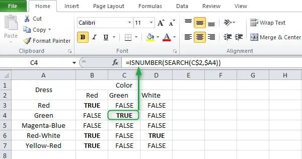
• But, there is a way out of this predicament. Instead of using that method, you should make a list of all the colors that are in the neighboring columns.

=ISNUMBER(SEARCH(C$2,$A4))

• In the formula that you just looked at, the value C$2 denotes the color that you want to look for, and the value $A4 indicates the cell where you want to look for it. Make any necessary adjustments to these mobile phone numbers.
• When you press Enter, the outcome will be shown as appropriate.

How do I style the output of the ISNUMBER function such that they are in color?

Do the following if you wish to modify the color of the ISNUMBER function result, which will result in TRUE appearing differently:

• To begin, choose all of the cells that will house either the YES or the FALSE answer.
• Now, under Styles, select Conditional Formatting, and then click the Create Rule button.
• Choose the second option, which is to format only the cells that include the content. Choose Particular Text, Contains from the menu that appears under Modify the Rule Description, and then enter TRUE into the form that appears underneath it. Check out the Snapshot that we have below

• After clicking the Format button, select a color from the drop-down selection that appears in the following dialog.

• After you click the OK button, you will notice that all of the cells that have the TRUE result will now be colored red (the chosen color).

With Excel, how can I search for a certain phrase or number?

There will be occasions in which you would wish to do a search on the Excel spreadsheet for a specific text or number. It may not be that difficult to locate that value in your excel file if it does not include a lot of information. Having a vast quantity of data, however, makes this more difficult to accomplish.

In that scenario, you can use the keyboard shortcut Ctrl + F and then put “to be searched item” into the box that says “Find what:.” Click the Find All button to retrieve each occurrence of the text or number that was searched for.

The first cell of all cells that contain the object that was searched for will have its contents highlighted automatically. Go to the tab labeled “Replace” and write the same thing into the box labeled “Replace with:” if you want the text that was searched for to be replaced with a different text.

If you want to make a change to only one cell, click the Replace button. Click the Replace all button to modify all of the values that contain the information that you looked for. Excel will immediately replace the selected text with the text that you want to use if you only wait a few seconds.

That sums it up well.

---

---